SpatialVista - Interactive Spatial Transcriptomics Visualization

Overview

SpatialVista is an interactive 2D/3D spatial transcriptomics visualization tool. Open an .h5ad file directly from the command line in a local browser, or embed the same interface in Jupyter Notebook/Lab.

🌐 Web and App Access

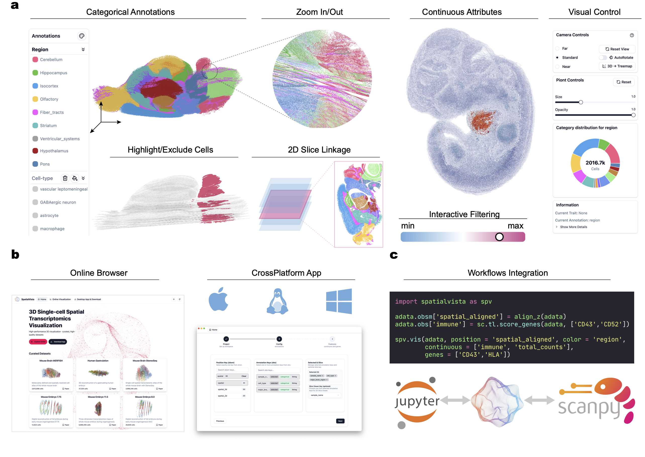
In addition to the Jupyter-based interface, SpatialVista is also available as:

• Web version: https://yanglab.westlake.edu.cn/spatialvista/vis
• Desktop Apps: https://yanglab.westlake.edu.cn/spatialvista/download

These options allow users to explore 3D spatial transcriptomics data without setting up a Python environment.

Note that the web/app versions support the same core visualization functionalities, while the Jupyter version enables seamless integration with analysis workflows.

✨ Key Features

• 🚀 High-Performance Rendering - WebGL-based 3D rendering supporting millions of cells
• 📊 Multi-Dimensional Data Display - Support for categorical annotations, continuous values, gene expression, and more
• 🎨 Interactive Controls - Real-time adjustment of colors, transparency, point size, and other parameters
• 🔬 2D/3D View Switching - Flexible switching between 3D point cloud and 2D slice views
• 🧬 Gene Expression Query - Quick visualization of spatial expression patterns for any gene
• 📐 Multiple Layout Modes - Support for original coordinates, 2D Treemap, histogram, and more
• 🎯 Precise Filtering - Filter data points by category, numerical range, and other conditions
• 💾 One-Click Screenshots - Easily save current views for publications and reports
• 🖥️ Local CLI Server - Open .h5ad files without writing Python or starting Jupyter
• 🪢 Lasso Selection - Select visible cells directly in either 2D or 3D views
• ↕️ Adjustable Slice Spacing - Expand or compress stacked sections along Z in 3D
• 🧭 Section Alignment - Translate, rotate, scale, flip, and align slices from annotations, tissue outlines, or both

🎯 Use Cases

SpatialVista is particularly suitable for:

• Spatial Transcriptomics Data Exploration - Visium, MERFISH, seqFISH, STARmap, and other technologies
• Single-Cell Spatial Data Analysis - Visualize spatial distribution of cell types
• Tissue Architecture Studies - Explore molecular features of tissue regions
• Gene Expression Pattern Analysis - View spatial expression of specific genes
• Data Quality Control - Quickly check data integrity and outliers

🚀 Quick Start

Dependencies:

• Python >= 3.10
• Tested on:
  • macOS 12.0+ (Intel/Apple Silicon)
  • Linux (Ubuntu 18.04+)
  • Windows (windows10/11)
• Recommended browsers: Chrome or other Chromium-based browsers (with WebGL support).

Installation

pip install spatialvista

Or run it without a permanent installation:

uvx spatialvista --input data.h5ad

Command-line usage

The shortest command automatically detects a common spatial coordinate key and categorical annotation:

spatialvista --input data.h5ad

SpatialVista starts a local server at http://127.0.0.1:8765 and opens your browser. Override inferred keys or preload additional data when needed:

spatialvista --input data.h5ad \
  --position spatial \
  --color celltype \
  --section slice_id \
  --annotations leiden,tissue_region \
  --continuous total_counts,n_genes_by_counts \
  --genes PECAM1,CD3E

Use spatialvista --help for options including --host, --port, --mode, --layer, and --no-browser. The default host is loopback-only, so data is not exposed to other machines.

Jupyter usage

Launch your jupyter notebook or jupyter lab. And play with SpatialVista!

jupyter-lab

import spatialvista as spv
import numpy as np

# Create minimal test data
class FakeAnnData:
    def __init__(self, n: int):
        self.obsm = {"spatial": np.random.rand(n, 3)}
        self.obs = {"celltype": np.random.choice(["A", "B", "C"], n)}
        self.var_names = []
        self.X = None
        self.n_obs = n
adata = FakeAnnData(n=10_000)

# Create visualization
spv.vis(adata, position="spatial", color="celltype")


import scanpy as sc
# Load yout real data
adata = sc.read_h5ad("spatial_data.h5ad")

# Create interactive visualization
spv.vis(
    adata,
    position="spatial",  # obsm key containing spatial coordinates
    color="celltype",    # Default annotation for coloring
    height=600               # Widget height in pixels
)

That's it! 🎉

More demo data for test

1. Cubic mock data: https://yanglab.westlake.edu.cn/gsmap3d/data/cube.h5ad
2. Mouse Brain data: https://yanglab.westlake.edu.cn/gsmap3d/data/mouse_brain_3_IQ.h5ad

📚 Core Features

1. Categorical Annotation Visualization

# Color by cell type
widget = spv.vis(
    adata,
    position="spatial",
    color="celltype",
    annotations=["leiden", "tissue_region"]  # Additional annotations to load
)

2. Continuous Value Visualization

# Visualize continuous values (e.g., QC metrics)
widget = spv.vis(
    adata,
    position="spatial",
    color="celltype",
    continuous=["total_counts", "n_genes"]  # Continuous value fields
)

3. Gene Expression Visualization

# View expression patterns of specific genes
widget = spv.vis(
    adata,
    position="spatial",
    color="celltype",
    genes=["Pecam1", "Cd3e", "Epcam"],  # Gene list
    layer="normalized"  # Optional: use specific layer if available
)

4. 2D/3D View Switching

# If data has section information, switch to 2D view in UI
widget = spv.vis(
    adata,
    position="spatial",
    color="celltype",
    section="slice_id",  # Section identifier field for section browser
)

When section is provided, the 3D Point Controls panel includes Slice spacing controls. Multiplier mode scales the original spacing (1.0× preserves it), while Fixed distance assigns an exact uniform Z distance such as 100 between adjacent section centers. Both modes preserve within-section Z variation.

The Section Alignment panel lets you choose reference and active slices and manually fine-tune XY translation, rotation, scale, and X/Y flipping. Translation uses a compact XY drag pad and rotation uses a direct manipulation dial; drag controls render immediately, while numeric values apply on Enter. Auto align supports annotation landmarks, complete tissue outlines, or a hybrid score that combines both. Batch workflows can align every section to the first section or align them sequentially as S1 → S2 → S3 → …. The outline search uses a bounded, downsampled boundary representation, while the hybrid mode exposes an annotation-weight control. Automatic scaling is opt-in and safely limited to avoid extreme estimates. In Jupyter, materialize the current result as a new AnnData coordinate matrix:

widget = spv.vis(
    adata,
    position="spatial",
    color="celltype",
    section="slice_id",
    annotations=["organ"],
)

# After aligning slices in the widget:
widget.apply_alignment(output_key="spatial_aligned")
# adata.obsm["spatial_aligned"] now contains the aligned 3D coordinates

The current JSON-compatible parameters are also available as widget.alignment_parameters and can be downloaded from the alignment panel.

🎨 Interactive Controls

Once displayed, the widget provides rich interactive controls for exploring your data:

• Navigate in 3D space (rotate, pan, zoom)
• Switch between annotations and customize colors
• Query continuous values and gene expression
• Filter by thresholds and hide specific categories
• Adjust visualization parameters (size, opacity, layout)
• Export screenshots

🤝 Contributing & Support

Issues and Pull Requests are welcome!

• GitHub: https://github.com/JianYang-Lab/spatial-vista-py
• Documentation: https://jianyang-lab.github.io/spatial-vista-py/

📄 License

SpatialVista is open-sourced under the MIT License.

---

Built by WenjieWei@YangLab