SMEARS is a modeling package. It takes observations processed through the FHD (Fast Holographic Deconvolution) software package (found here: https://github.com/EoRImaging/FHD) and converts these observations into models for sources. These models consider the potential of these sources to be diffuse and can either create extended models for diffuse sources or recognize and model sources as point-like. The code also handles situations where sources have both diffuse and point like structure, producing an extended model for the diffuse structure and a point model for point-like structure.
SMEARS is made up of several different functions, each designed to make the process of searching for sources, modeling them, and outputting catalog files as intuitive as possible. This is done through several steps:
- Building a Pandas DataFrame contianing the GLEAM objects from an input GLEAM catlog and the sources identified in the FHD processed observation files. Each row in this DataFrame represents an object from the GLEAM file and it's data from each observation. Objects not observed are indicated by a 0 magnitude.
- Identify sources that may benefit from a more complete model. This can be done in many ways, but the easiest may be to use the source_search function, which allows a user to specify things like minimum magnitude in Jy, a block of sky to search, and several other parameters that may be helpful to consider.
- Models can then be generated for such sources. This process is a bit more complex and is detailed below.
- Writing out a new file in the SkyModel format from the pyradiosky libraray containing the original GLEAM catalog but with the new sources replacing the old GLEAM objects. This is accomplished with the gen_SkyModel function.
##The Modeling Technique
The process by which these models are generated takes place through several functions. The model generation sequence can be initiated by calling the gen_SkyModel function and feeding it a list of sources to model or by callin the create_plots function on a single source. Either of these methods will initiate the same sequence of code to generate the source models.
This code is extensively doccumented in the SMEARS.py file. For a detailed look at how this code functions, I reccomend looking through that file. Here, I will give a short overview, in simple terms, of exactly what this code does. I'll talk about the code here with the aim of someone reading this README coming out of it with a good sense of what it is doing without having to look at any code or understand low frequency radio astrophysics.
First, we need to start with the probelm. This work focuses on radio data taken across the entire sky at very low frequencies (around 8 GHz). We are concerned with a signal from the very early universe, the 21cm signal of neutral hydrogen that populated the universe before the first stars and galaxies. This means we have all the radio-bright astrophysical "stuff" in between us and this signal. We need incredibly accurate models for these sources in order to calibrate around them and subtract them from the overall data.
Previous work has assumed that these sources are point-like. As I've shown repeatedly with this work, that assumption is far from the truth. My personal best guess is that at least a third of radio-bright objects in our data are not points. A lot of these objects are distant, active black holes spewing out jets that turn them in to hour-glass shaped sources. Modeling sources like this as points can really severly contaminate observations. Our goal was to find a better way to generate lots of models for individual sources without assuming this point-like structure.
I mentioned that the data I work with is an output for something called FHD. This is the Fast (it is not fast) Holographic (I've spent years trying to get someone to explain to me why this is holographic. No one can.) Deconvolution (it is a deconvolution!). It works by taking an ammount of light from a part of the telscope observation that it decides is a source and sort of pull the light together in to a point source. If you've got a mathy background, the deconvolution algorithm is collapsing the flux into delta functions in an attempt to resolve the source. When this encounters a non-pointlike source, this does not work! FHD spits out an array of these points it has atttempted to collect, each with a corresponding flux. You've read this far so I think you desrve a litttle picture at this point. HEre is an example of what a source looks like when we deconvolve it into points. Each of the colors here is a different observation of the source.
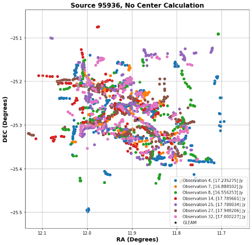
That single black star in the center os how previous code would model this source. You don't need to be a radio astronomer to tell that this is a poor representation of the source.
The goal is to turn these individual point arrays into something that looks like the sources so we can subtract it from the data and calibrate asound it. I'll talk you through the modeling algorithm next which takes those point arrays and turns them in to a model that looks like this:
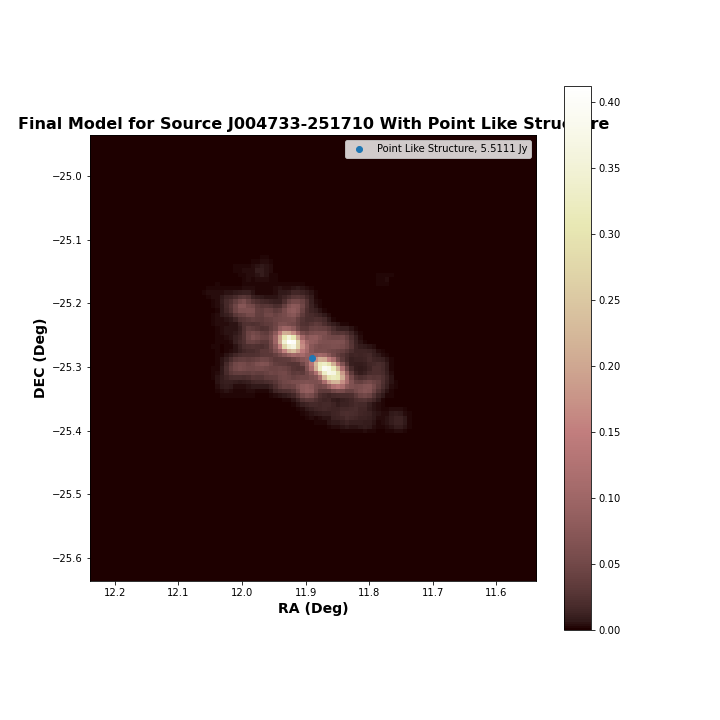
Wow so pretty. But how did I do it? First we need to consider the observations individualy. As you can see from the model I showed, a lot of these sources really do have some point-like portion to them. In this example, it is a very bright spot right in the center of the object. These are (almost always) bright, active black holes at the center of galaxies, or even just very bright black holed spewing out radiation. We need to find somewhere between an aproach that just gives up and treats the source as point-like and an aproach that washes out a really point-like portion of the source. To handle this, we lay several "test rings" all over the image. If the ammount of light within a test ring exceeded some arbitrary total percentage of the light of the source, we take all points that lie within that ring and pull them out of the source entirely, assigning a point to where they were in the original array. This involves actually editing our point arrays as we iterate over them with these rings. This ultimately seperates the observation in to light that contributes to point-like structure and light that contributes to diffuse structure.
Our next step is to treat this diffuse structure as diffuse! We overlay a grid and put our remaining points on top of it. If you are not mathy, picture taking a bunch of these points each with some brightness and using a "blur" tool in photoshop to turn them in to blurs instead of points. If you are mathy, I take each of these points and smooth them as a gaussian over a matrix where the gaussian power is the flux of a given point and the total matrix flux is normalized to the total flux of the original input array. Now we have several matricies, each corresponding to an individual observation of the source, and point-like structure for each of these observations. I then take these 'point-like' components of the individual observations and put them through another round of this ring placement editing. This portion of the code decides if individual point-like contributions from the observations can be combined into an overall point-like portion of the source. If they can't (if the point-like portion is just in one observation, if the point-like part is not consistent across observations...), we throw these points back in to the original observation before it goes through the smoothing process that turned the diffuse observation into image-like data.
Next, we need to commbine the individual observations together to make a final model. The point-like components are already combined, but the image-like data needs some more consideration. For the source above, here is what those individual images looked like before I combined them:
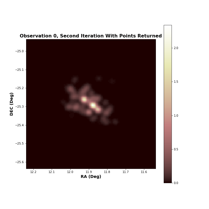
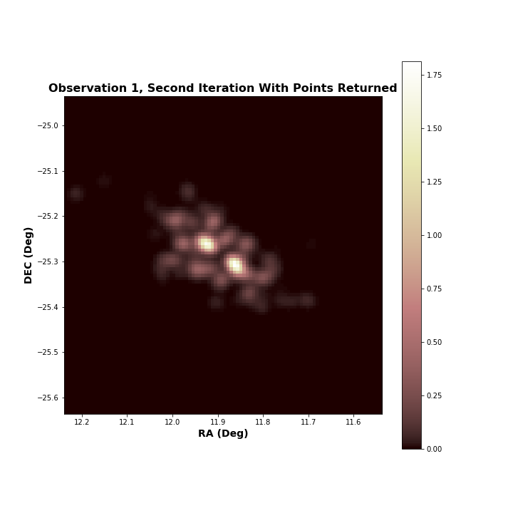
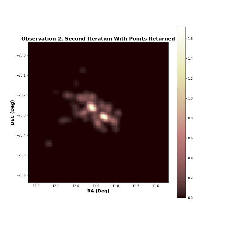
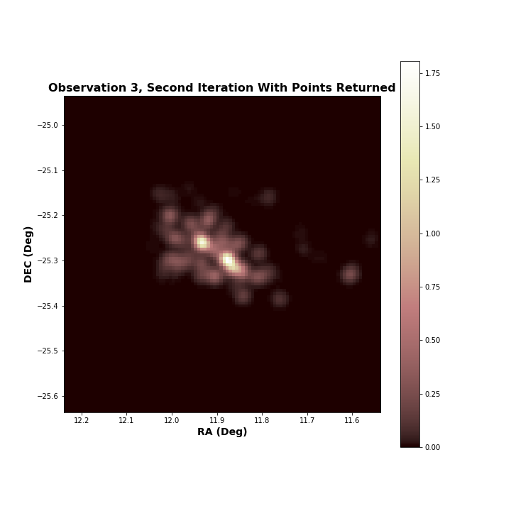
You can see that each of them vary a whole lot between observations. You may have already learned that by staring at the first plot. This is primarily due to the ionosphere layer of the Earth's atmosphere. This layer has a lot of bubling and activity that interferes with radio wavelength data and jumbles observations. The best way around this is to take data on the far side of the moon. That's outside the scope of this project, so we are forced to come up with other solutions. The most effective way to combat this is to combine as many images for a sources as possible. We then overlay all these images on top of each other and take a median value for each pixel in the image. This gets rid of fluctuations that occured just on one imaage and keeps areas of the source that are consistently bright across observatiosn. After this, we finally arive at the image I showed.
This work needs some final resolving things. The code is built so that it can be run on several sources at once and generate sky catalogs that can be used in calibration. Calibrating the data is fairly intensive, so it has only been tested once. I simply replaced one source with my updated model and looked at how this changed the quality of the image.
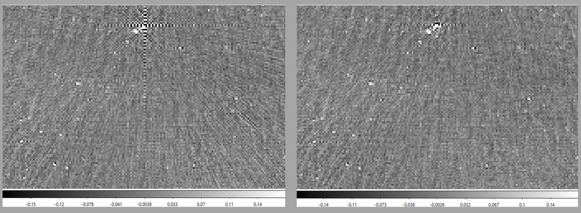
The left pannel here is the original observation with the previous calibration catalogs applied. There is something going on at the center of a cross you can make out. This distortion at the center is what happens when calibration fails. Essentially, it is punching a hole in the image. Errors like this propogate through the observation, and a few other artifacts pop up. In the escond image, I just replaced the source at the center of this cross with my updated model for it. You can see the the cross is a lot less prevalent and faint lines that are extending out from the source in the original image are mitigated. This shows me that the improved model has a lot of potential for image quality improvement.
As it stands, I have not worked on this code for quite some time. I have seen a lot of the low-frequency radio sky and that has been exciting. I'll include here some fun objects that I have found, most of which are not identified in any other catalogs I have found. I have sky maps of more sources than I could ever hope to include here and nothing to do with them. If you have any interest in the low frequency radio sky in the southern hemisphere, I am happy to share them. Here are some of the prettier things I have seen in my modeling searches.
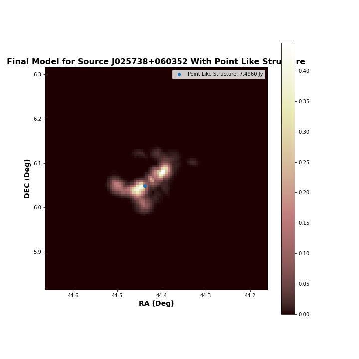
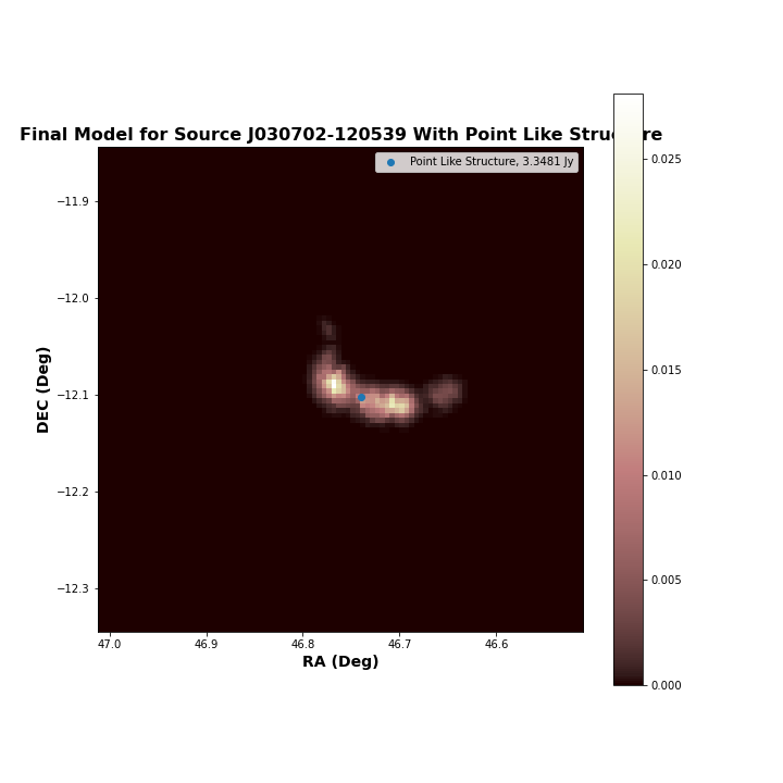
Almost all the radio-bright sources look like this:
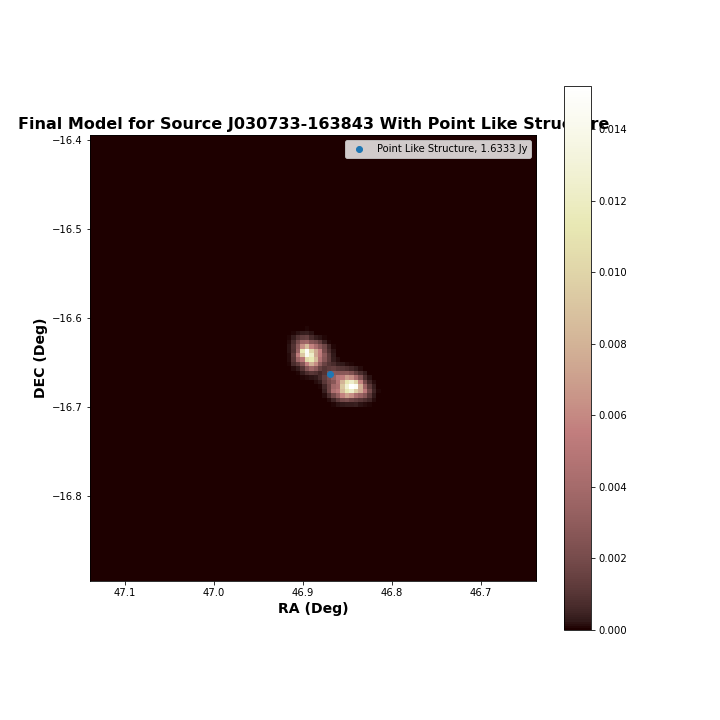
That makes sense. It's a black hole with bright jets. I'd guess something like 80% of diffuse sources look like this. But some lobed sources are a bit weird. Like this one that doesn't seem to have a bright center:
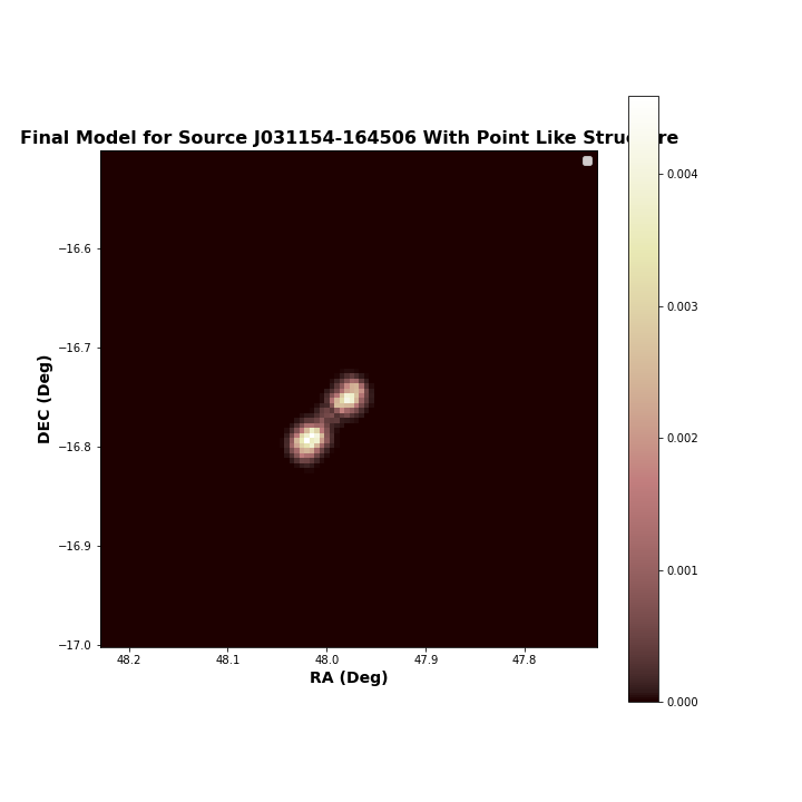
Some are even offset (a factor of viewing angle):
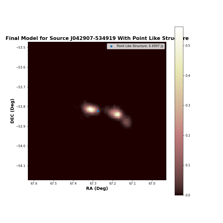
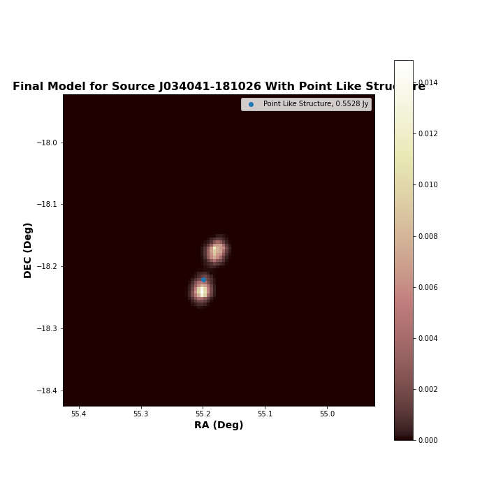
Some even come in pairs:
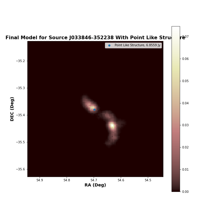
This project was intended to be expanded into my PhD work during my time at Brown. I ultimetely chose to leave the department, and this project got abandoned with my departure. If you have stumbled on this repository because you think the work may be useful, I reccomend downloading the SMEARS.py with the jupyter notebook titles "Active Work" and going from there. There are a lot of functions that depend on each other and several decisions that need to be made when running this code, and I am fairly responsive over email (my most current email is in my Github bio). Don't hesitiate to reach out if you find yourself here. This code took years of hard work and I care for it very much, I'd be thrilled if someone used it.